42 KiB
Supply and demand
An initial orientation to the supply and demand options in the model PyPSA-Eur-Sec can be found in the description of the model PyPSA-Eur-Sec-30 in the paper Synergies of sector coupling and transmission reinforcement in a cost-optimised, highly renewable European energy system (2018). The latest version of PyPSA-Eur-Sec differs by including biomass, industry, industrial feedstocks, aviation, shipping, better carbon management, carbon capture and usage/sequestration, and gas networks.
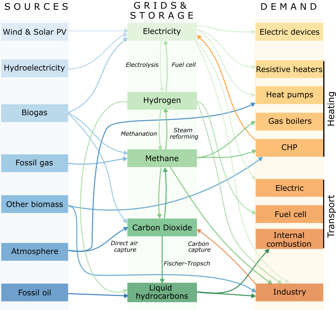
The basic supply (left column) and demand (right column) options in the model are described in this figure:
Electricity supply and demand
Electricity supply and demand follows the electricity generation and transmission model PyPSA-Eur, except that hydrogen storage is integrated into the hydrogen supply, demand and network, and PyPSA-Eur-Sec includes CHPs.
Unlike PyPSA-Eur, PyPSA-Eur-Sec does not distribution electricity demand for industry according to population and GDP, but uses the geographical data from the Hotmaps Industrial Database.
Also unlike PyPSA-Eur, PyPSA-Eur-Sec subtracts existing electrified heating from the existing electricity demand, so that power-to-heat can be optimised separately.
The remaining electricity demand for households and services is distributed inside each country proportional to GDP and population.
Heat demand
Building heating in residential and services sectors is resolved regionally, both for individual buildings and district heating systems, which include different supply options [To do:link to next section] Annual heat demands per country are retrieved from JRC-IDEES and split into space and water heating. For space heating, the annual demands are converted to daily values based on the population-weighted Heating Degree Day (HDD) using the atlite tool, where space heat demand is proportional to the difference between the daily average ambient temperature (read from ERA5) and a threshold temperature above which space heat demand is zero. A threshold temperature of 15 °C is assumed by default. The daily space heat demand is distributed to the hours of the day following heat demand profiles from BDEW. These differ for weekdays and weekends/holidays and between residential and services demand.
Space heating
The space heating demand can be exogenously reduced by retrofitting measures that improve the buildings’ thermal envelopes [Refer to PyPSA-Eur-Sec Config file, line 212.
System Message: ERROR/3 (<stdin>, line 48)
Unknown directive type "literalinclude".
.. literalinclude:: ../config.default.yaml
    :language: yaml
    :lines: 212
Co-optimsing of building renovation is also possible, if it is activated in the config file. Renovation of the thermal envelope reduces the space heating demand and is optimised at each node for every heat bus. Renovation measures through additional insulation material and replacement of energy inefficient windows are considered. In a first step, costs per energy savings are estimated in build_retro_cost.py. They depend on the insulation condition of the building stock and costs for renovation of the building elements. In a second step, for those cost per energy savings two possible renovation strengths are determined: a moderate renovation with lower costs, a lower maximum possible space heat savings, and an ambitious renovation with associated higher costs and higher efficiency gains. They are added by step-wise linearisation in form of two additional generations in prepare_sector_network.py. Further information are given in the publication :
System Message: ERROR/3 (<stdin>, line 56)
Unexpected indentation.Mitigating heat demand peaks in buildings in a highly renewable European energy system, (2021).
Water heating
Hot water demand is assumed to be constant throughout the year.
Urban and rural heating
System Message: WARNING/2 (<stdin>, line 5); backlink
Duplicate explicit target name: "config file".For every country, heat demand is split between low and high population density areas. These country-level totals are then distributed to each region in proportion to their rural and urban populations respectively. Urban areas with dense heat demand can be supplied with large-scale district heating systems. The percent of urban heat demand that can be supplied by district heating networks as well as lump-sum losses in district heating systems is exogenously determined in the Config file.
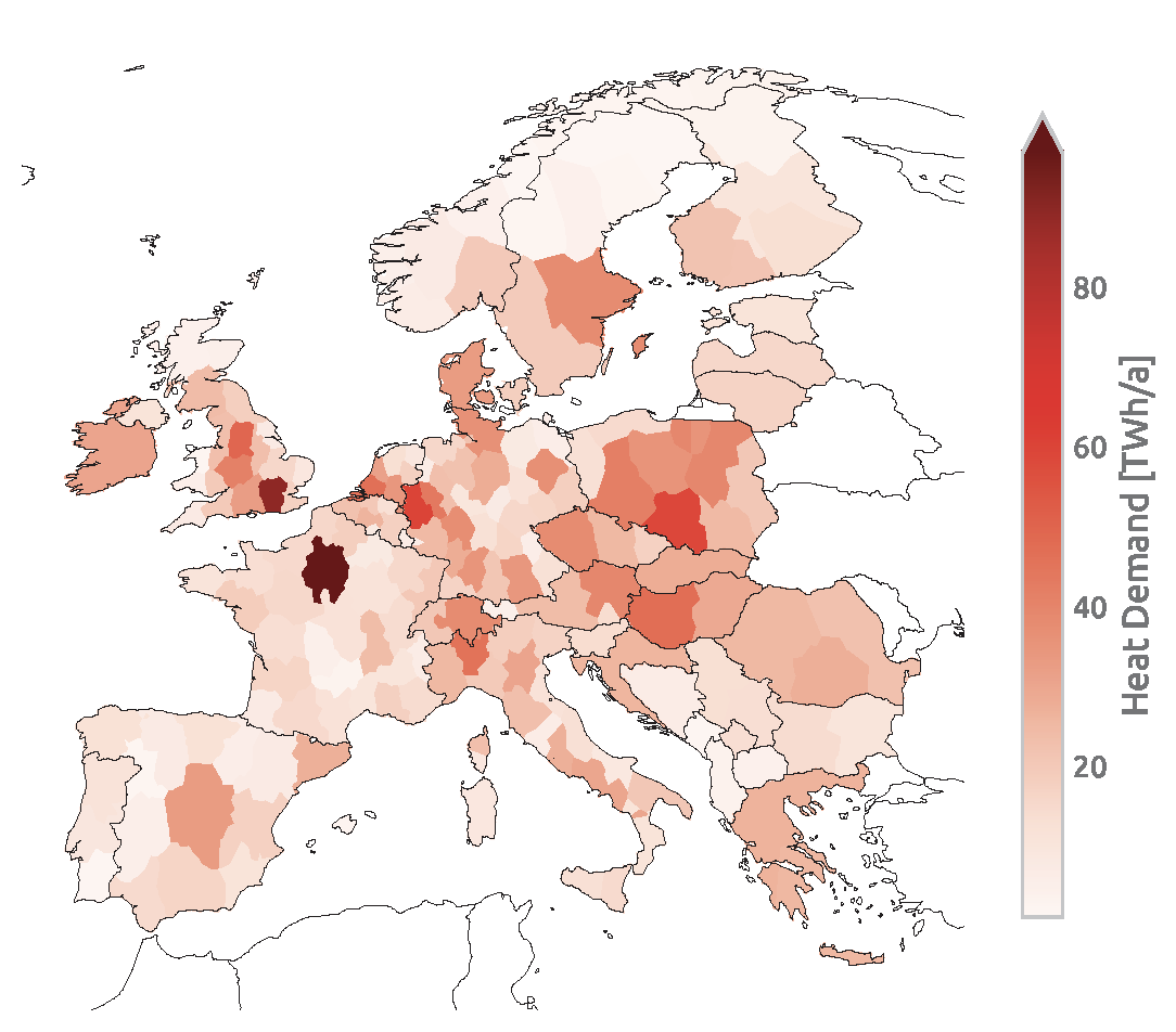
Cooling demand Cooling is electrified and is included in the electricity demand. Cooling demand is assumed to remain at current levels. An example of regional distribution of the total heat demand for network 181 regions is depicted below.
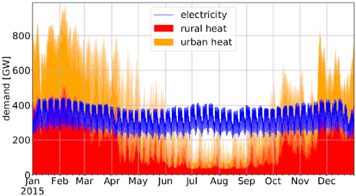
As below figure shows, the current total heat demand in Europe is similar to the total electricity demand but features much more pronounced seasonal variations. The current total building heating demand in Europe adds up to 3084 TWh/a of which 78% occurs in urban areas.
In practice, in PyPSA-Eur-Sec, there are heat demand buses to which the corresponding heat demands are added.
- Urban central heat: large-scale district heating networks in urban areas with dense heat population. Residential and services demand in these areas are added as demands to this bus
- Residential urban decentral heat: heating for residential buildings in urban areas not using district heating
- Services urban decentral heat: heating for services buildings in urban areas not using district heating
- Residential rural heat: heating for residential buildings in rural areas with low population density.
- Services rural heat: heating for residential services buildings in rural areas with low population density. Heat demand from agriculture sector is also included here.
Heat supply
Different supply options are available depending on whether demand is met centrally through district heating systems, or decentrally through appliances in individual buildings.
Urban central heat
For large-scale district heating systems the following options are available: combined heat and power (CHP) plants consuming gas or biomass from waste and residues with and without carbon capture (CC), large- scale air-sourced heat pumps, gas and oil boilers, resistive heaters, and fuel cell CHPs. Additionally, waste heat from the Fischer-Tropsch and Sabatier processes for the production of synthetic hydrocarbons can supply district heating systems.
Residential and Urban decentral heat
Supply options in individual buildings include gas and oil boilers, air- and ground-sourced heat pumps, resistive heaters, and solar thermal collectors. Ground-source heat pumps are only allowed in rural areas because of space constraints. Thus, only air- source heat pumps are allowed in urban areas. This is a conservative assumption, since there are many possible sources of low-temperature heat that could be tapped in cities (e.g. waste water, ground water, or natural bodies of water). Costs, lifetimes and efficiencies for these technologies are retrieved from the Technology-data repository.
Below are more detailed explanations for each heating supply component, all of which are modeled as Links. in PyPSA-Eue-Sec.
Large Combined Heat and Power plants are included in the model if it is specified in the config file..
CHPs are based on back pressure plants operating with a fixed ratio of electricity to heat output. The efficiencies of each are given on the back pressure line, where the back pressure coefficient cb is the electricity output divided by the heat output. (For a more complete explanation of the operation of CHPs refer to the study by Dahl et al. : Cost sensitivity of optimal sector-coupled district heating production systems.
PyPSA-Eur-Sec includes CHP plants fueled by methane and solid biomass from waste and residues. Hydrogen fuel cells also produce both electricity and heat.
The methane CHP is modeled on the Danish Energy Agency (DEA) “Gas turbine simple cycle (large)” while the solid biomass CHP is based on the DEA’s “09b Wood Pellets Medium”. For biomass CHP, cb = 0.46 , whereas for gas CHP, cb = 1.
NB: The old PyPSA-Eur-Sec-30 model assumed an extraction plant (like the DEA coal CHP) for gas which has flexible production of heat and electricity within the feasibility diagram of Figure 4 in the study by Brown et al. We have switched to the DEA back pressure plants since these are more common for smaller plants for biomass, and because the extraction plants were on the back pressure line for 99.5% of the time anyway. The plants were all changed to back pressure in PyPSA-Eur-Sec v0.4.0.
Micro-CHP
Pypsa-eur-sec allows individual buildings to make use of micro gas CHPs that are assumed to be installed at the distribution grid level.
Heat pumps
The coefficient of performance (COP) of air- and ground-sourced heat pumps depends on the ambient or soil temperature respectively. Hence, the COP is a time-varying parameter[refer to Config file). Generally, the COP will be lower during winter when temperatures are low. Because the ambient temperature is more volatile than the soil temperature, the COP of ground-sourced heat pumps is less variable. Moreover, the COP depends on the difference between the source and sink temperatures:
$$ Δ T = T_(sink) − T_(source) $$
System Message: WARNING/2 (<stdin>, line 5); backlink
Duplicate explicit target name: "config".For the sink water temperature Tsink we assume 55 °C [Config file] For the time- and location-dependent source temperatures Tsource, we rely on the ERA5 reanalysis weather data. The temperature differences are converted into COP time series using results from a regression analysis performed in the study by Stafell et al.. For air-sourced heat pumps (ASHP), we use the function:
$$ COP (Δ T) = 6.81 + 0.121Δ T + 0.000630.Δ T^2; $$
for ground-sourced heat pumps (GSHP), we use the function:
$$ COP(Δ T) = 8.77 + 0.150Δ T + 0.000734Δ T^2 $$
Resistive heaters
Can be activated in Config from the boilers option Resistive heaters produce heat with a fixed conversion efficiency (refer to Technology-data repository ).
Gas, oil, and biomass boilers
Can be activated in Config from the boilers , oil boilers , and biomass boiler option. Similar to resistive heaters, boilers have a fixed efficiency and produce heat using gas ,oil or biomass.
Solar thermal collectors
Can be activated in the Config file from the solar_thermal option. Solar thermal profiles are built based on weather data and also have the options for setting the sky model and the orientation of the panel in the Config file, which are then used by the atlite tool to calculate the solar resource time series.
Waste heat from Fuel Cells, Methanation and Fischer-Tropsch plants
Waste heat from fuel cells in addition to processes like Fischer-Tropsch , methanation, and Direct Air Capture (DAC) is dumped into district heating networks.
Existing heating capacities and decommissioning
For the myopic transition paths, capacities already existing for technologies supplying heat are retrieved from “Mapping and analyses of the current and future (2020 - 2030)” . For the sake of simplicity, coal, oil and gas boiler capacities are assimilated to gas boilers. Besides that, existing capacities for heat resistors, air-sourced and ground-sourced heat pumps are included in the model. For heating capacities, 25% of existing capacities in 2015 are assumed to be decommissioned in every 5-year time step after 2020.
Thermal Energy Storage
Activated in Config from the tes option.
Thermal energy can be stored in large water pits associated with district heating systems and individual thermal energy storage (TES), i.e., small water tanks. Water tanks are modeled as stores. A thermal energy density of 46.8 kWhth/m3 is assumed, corresponding to a temperature difference of 40 K. The decay of thermal energy in the stores: 1-exp(-1/24τ) is assumed to have a time constant of t=180 days for central TES and t=3 days for individual TES, both modifiable through tes_tau in Config file. Charging and discharging efficiencies are 90% due to pipe losses.
Retrofitting of the thermal envelope of buildings
System Message: WARNING/2 (<stdin>, line 5); backlink
Duplicate explicit target name: "config".Co-optimising building renovation is only enabled if in the config file. To reduce the computational burden, default setting is set as false
Renovation of the thermal envelope reduces the space heating demand and is optimised at each node for every heat bus. Renovation measures through additional insulation material and replacement of energy inefficient windows are considered.
System Message: WARNING/2 (<stdin>, line 5); backlink
Duplicate explicit target name: "build_retro_cost.py".System Message: WARNING/2 (<stdin>, line 5); backlink
Duplicate explicit target name: "prepare_sector_network.py".In a first step, costs per energy savings are estimated in the build_retro_cost.py script. They depend on the insulation condition of the building stock and costs for renovation of the building elements. In a second step, for those cost per energy savings two possible renovation strengths are determined: a moderate renovation with lower costs and lower maximum possible space heat savings, and an ambitious renovation with associated higher costs and higher efficiency gains. They are added by step-wise linearisation in form of two additional generations in the prepare_sector_network.py script.
Settings in the config.yaml concerning the endogenously optimisation of building renovation include cost factor, interest rate, annualised cost, tax weighting, and construction index.
Further information are given in the study by Zeyen et al. : Mitigating heat demand peaks in buildings in a highly renewable European energy system, (2021).
Hydrogen demand
Hydrogen is consumed in the industry sector (link to industry) to produce ammonia [link to ammonia industry section] and direct reduced iron (DRI) [link to DRI industry section]. Hydrogen is also consumed to produce synthetic methane [link to section “Methane supply”] and liquid hydrocarbons [link to fossil-oil based supply”] which have multiple uses in industry and other sectors. Hydrogen is also used for transport applications (link to transport), where it is exogenously fixed. It is used in heavy-duty land transport and as liquified hydrogen in the shipping sector [add link to shipping sector]. Furthermore, stationary fuel cells may re-electrify hydrogen (with waste heat as a byproduct) to balance renewable fluctuations [Add a link to the section where we describe the Electricity sector and how storage is modelled there]. The waste heat from the stationary fuel cells can be used in district-heating systems.
Hydrogen supply
Today, most of the H2 consumed globally is produced from natural gas by steam methane reforming (SMR)
$$ CH_4 + H_2O → CO + 3H_2 $$
combined with a water-gas shift reaction
$$ CO + H_2O → CO_2 + H_2 $$
SMR is included here. PyPSA-Eur-Sec allows this route of H2 production with and without [carbon capture (CC)] (Link to section on Carbon Capture Storage and Utilization). These routes are often referred to as blue and grey hydrogen. Here, methane input can be both of fossil or synthetic origin.
Green hydrogen can be produced by electrolysis to split water into hydrogen and oxygen
$$ 2H_2O → 2H_2 + O_2 $$
For the electrolysis, alkaline electrolysers are chosen since they have lower cost and higher cumulative installed capacity than polymer electrolyte membrane (PEM) electrolysers. The techno-economic assumptions are taken from the technology-data repository. Waste heat from electrolysis is not leveraged in the model.
Transport
System Message: WARNING/2 (<stdin>, line 5); backlink
Duplicate explicit target name: "config file".Hydrogen is transported by pipelines. H2 pipelines are endogenously generated, either via a greenfield H2 network, or by retrofitting natural gas pipelines). Retrofitting is implemented in such a way that for every unit of decommissioned gas pipeline, a share (60% is used in [link to H2 backbone study]) of its nominal capacity (exogenously determined in the config file.) is available for hydrogen transport. When the gas network is not resolved, this input denotes the potential for gas pipelines repurposed into hydrogen pipelines. New pipelines can be built additionally on all routes where there currently is a gas or electricity network connection. These new pipelines will be built where no sufficient retrofitting options are available. The capacities of new and repurposed pipelines are a result of the optimisation.
Storage
Hydrogen can be stored in overground steel tanks or underground salt caverns. For the latter, energy storage capacities in every country are limited to the potential estimation for onshore salt caverns within 50 km of shore to avoid environmental issues associated with brine solution disposal. Underground storage potentials for hydrogen in European salt caverns is acquired from Caglayan et al.
Methane demand
Methane is used in individual and large-scale gas boilers, in CHP plants with and without carbon capture, in OCGT and CCGT power plants, and in some industry subsectors for the provision of high temperature heat[LINK TO INDUSTRY OVERVIEW]. Methane is not used in the trans- port sector because of engine slippage.
Methane supply
In addition to methane from fossil origins, the model also considers biogenic and synthetic sources. The gas network can either be modeled, or it can be assumed that gas transport is not limited. If gas infrastructure is regionally resolved, fossil gas can enter the system only at existing and planned LNG terminals, pipeline entry-points, and intra- European gas extraction sites, which are retrieved from the SciGRID Gas IGGIELGN dataset and the GEM Wiki. Biogas can be upgraded to methane. Synthetic methane can be produced by processing hydrogen and captures CO2 in the Sabatier reaction
$$ CO_2 + 4H_2 → CH_4 + 2H_2O $$
Direct power-to-methane conversion with efficient heat integration developed in the HELMETH project is also an option. The share of synthetic, biogenic and fossil methane is an optimisation result depending on the techno-economic assumptions.
Methane transport
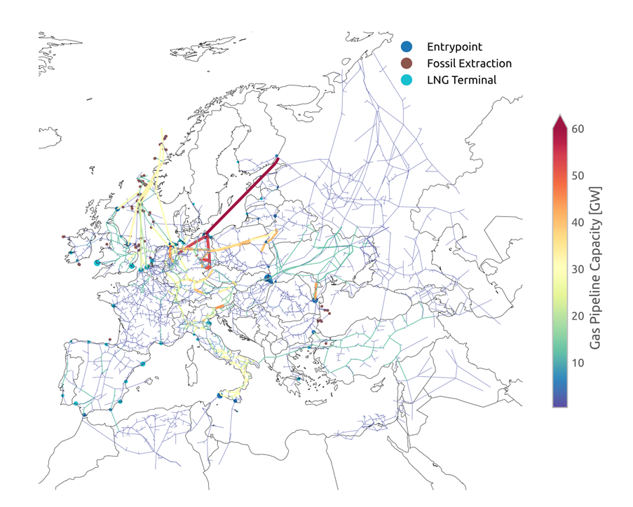
The existing European gas transmission network is represented based on the SciGRID Gas IGGIELGN dataset. This dataset is based on compiled and merged data from the ENTSOG maps and other publicly available data sources. It includes data on the capacity, diameter, pressure, length, and directionality of pipelines. Missing capacity data is conservatively inferred from the pipe diameter following conversion factors derived from an EHB report. The gas network is clustered to the selected number of model regions. Gas pipelines can be endogenously expanded or repurposed for hydrogen transport. Gas flows are represented by a lossless transport model. Methane is assumed to be transmitted without cost or capacity constraints because future demand is predicted to be low compared to available transport capacities.
The following figure shows the unclustered European gas transmission network based on the SciGRID Gas IGGIELGN dataset. Pipelines are color-coded by estimated capacities. Markers indicate entry-points, sites of fossil resource extraction, and LNG terminals.
Biomass Supply
System Message: WARNING/2 (<stdin>, line 5); backlink
Duplicate explicit target name: "here".Biomass supply potentials for each European country are taken from the JRC ENSPRESO database where data is available for various years (2010, 2020, 2030, 2040 and 2050) and scenarios (low, medium, high). No biomass import from outside Europe is assumed. More information on the data set can be found here.
Biomass demand
System Message: WARNING/2 (<stdin>, line 5); backlink
Duplicate explicit target name: "here".Biomass supply potentials for every NUTS2 region are taken from the JRC ENSPRESO database where data is available for various years (2010, 2020, 2030, 2040 and 2050) and different availability scenarios (low, medium, high). No biomass import from outside Europe is assumed. More information on the data set can be found here. The data for NUTS2 regions is mapped to PyPSA-Eur-Sec model regions in proportion to the area overlap.
System Message: WARNING/2 (<stdin>, line 5); backlink
Duplicate explicit target name: "here".The desired scenario can be selected in the pypsa-eur-sec configuration. The script for building the biomass potentials from the JRC ENSPRESO data base is located here. Consult the script to see the keywords that specify the scenario options.
The configuration also allows the user to define how the various types of biomass are used in the model by using the following categories: biogas, solid biomass, and not included.Feedstocks categorized as biogas, typically manure and sludge waste, are available to the model as biogas, which can be upgraded to biomethane. Feedstocks categorized as solid biomass, e.g. secondary forest residues or municipal waste . are available for combustion in combined-heat-and power (CHP) plants and for medium temperature heat (below 500 °C) applications in industry. It can also converted to gas or liquid fuels.
Feedstocks labeled as not included are ignored by the model.
A typical use case for biomass would be the medium availability scenario for 2030 where only residues from agriculture and forestry as well as biodegradable municipal waste are considered as energy feedstocks. Fuel crops are avoided because they compete with scarce land for food production, while primary wood, as well as wood chips and pellets, are avoided because of concerns about sustainability. See the supporting materials of the paper for more details.
Solid biomass conversion and use
Solid biomass can be used directly to provide process heat up to 500˚C in the industry. It can also be burned in CHP plants and boilers associated with heating systems. These technologies are described elsewhere [link to heat and industry sections].
System Message: WARNING/2 (<stdin>, line 5); backlink
Duplicate explicit target name: "config file".Solid biomass can be converted to syngas if the option is enabled in the config file. In this case the model will enable the technology BioSNG both with and without the option for carbon capture [link to technology data].
Liquefaction of solid biomass can be enabled allowing the model to convert it into liquid hydrocarbons that can replace conventional oil products. This technology also comes with and without carbon capture [link to technology data].
Transport of solid biomass
System Message: WARNING/2 (<stdin>, line 5); backlink
Duplicate explicit target name: "here".The transport of solid biomass can either be assumed unlimited between countries or it can be associated with a country specific cost per MWh/km. In the config file these options are toggled here. If the option is off, use of solid biomass is transport. If it is turned on, a biomass transport network will be created between all nodes. This network resembles road transport of biomass and the cost of transportation is a variable cost which is proportional to distance and a country specific cost per MWh/km. The latter is estimated from the country specific costs per ton/km used in the publication “The JRC-EU-TIMES model. Bioenergy potentials for EU and neighbouring countries”.
Biogas transport and use
Biogas will be aggregated into a common European resources if a gas network is not modeled explicitly, i.e., the gas_network option is set to false. If, on the other hand, a gas network is included, the biogas potential will be associated with each node of origin. The model can only use biogas by first upgrading it to natural gas quality [link to tech description] (bio methane) which is fed into the general gas network.
Oil-based products demand
System Message: WARNING/2 (<stdin>, line 298)
Title underline too short.
Oil-based products demand
========================
Naphtha is used as a feedstock in the chemicals industry[LINK TO CHEMICAL INDUSTRY]. Furthermore, kerosene is used as transport fuel in the aviation sector[LINK TO AVIATION SECTOR]. Non-electrified agriculture machinery also consumes gasoline. Land transport [LINK TO LAND TRANSPORT] that is not electrified or converted into using H2-fuel cells also consumes oil-based products. While there is regional distribution of demand, the carrier is copperplated in the model, which means that transport costs and constraints are neglected.
Oil-based products supply
System Message: WARNING/2 (<stdin>, line 304)
Title underline too short.
Oil-based products supply
========================
Oil-based products can be either of fossil origin or synthetically produced by combining H2 [link to hydrogen] and captured CO2 [link to carbon capture] in Fischer-Tropsch plants
$$ 𝑛CO+(2𝑛+1)H_2 → C_{n}H_{2n + 2} +𝑛H_2O $$
System Message: WARNING/2 (<stdin>, line 5); backlink
Duplicate explicit target name: "technology-data repository".with costs as included from the technology-data repository. The waste heat from the Fischer-Tropsch process is supplied to district heating networks. The share of fossil and synthetic oil is an optimisation result depending on the techno-economic assumptions.
Oil-based transport
Liquid hydrocarbons are assumed to be transported freely among the model region since future demand is predicted to be low, transport costs for liquids are low and no bottlenecks are expected.
Industry demand
Industry demand is split into a dozen different sectors with specific energy demands, process emissions of carbon dioxide, as well as existing and prospective mitigation strategies.
Subsection overview (link to section overview) provides a general description of the modelling approach for the industry sector. The following subsections describe the current energy demands, available mitigation strategies, and whether mitigation is exogenously fixed or co-optimised with the other components of the model for each industry subsector in more detail. See details for Iron and Steel (link to subsection Iron and Steel), Chemicals Industry (link to subsection Chemicals Industry), Ammonia (link to subsection Ammonia), Non-metallic Mineral products (link to subsection Non-metallic products), Non-ferrous Metals (link to subsection Non-ferrous Metals), Other Industry Subsectors (link to subsection Other Industry Subsectors).
Overview
Greenhouse gas emissions associated with industry can be classified into energy-related and process-related emissions. Today, fossil fuels are used for process heat energy in the chemicals industry, but also as a non-energy feedstock for chemicals like ammonia (NH3), ethylene (C2H4) and methanol (CH3OH). Energy-related emissions can be curbed by using low-emission energy sources. The only option to reduce process-related emissions is by using an alternative manufacturing process or by assuming a certain rate of recycling so that a lower amount of virgin material is needed.
The overarching modelling procedure can be described as follows. First, the energy demands and process emissions for every unit of material output are estimated based on data from the JRC-IDEES database and the fuel and process switching described in the subsequent sections. Second, the 2050 energy demands and process emissions are calculated using the per-unit-of-material ratios based on the industry transformations and the country-level material production in 2015, assuming constant material demand.
Missing or too coarsely aggregated data in the JRC-IDEES database is supplemented with additional datasets: Eurostat energy balances, United States, Geological Survey for ammonia production, DECHEMA for methanol and chlorine, and national statistics from Switzerland.
Where there are fossil and electrified alternatives for the same process (e.g. in glass manufacture or drying), we assume that the process is completely electrified. Current electricity demands (lighting, air compressors, motor drives, fans, pumps) will remain electric. Processes that require temperatures below 500 °C are supplied with solid biomass, since we assume that residues and wastes are not suitable for high-temperature applications. We see solid biomass use primarily in the pulp and paper industry, where it is already widespread, and in food, beverages and tobacco, where it replaces natural gas. Industries which require high temperatures (above 500 °C), such as metals, chemicals and non-metallic minerals are either electrified where suitable processes already exist, or the heat is provided with synthetic methane.
Hydrogen for high-temperature process heat is not part of the model currently.
Where process heat is required, our approach depends on the necessary temperature. For example, due to the high share of high-temperature process heat demand (see Naegler et al. and Rehfeldt el al.), we disregard geothermal and solar thermal energy as sources for process heat since they cannot attain high-temperature heat.
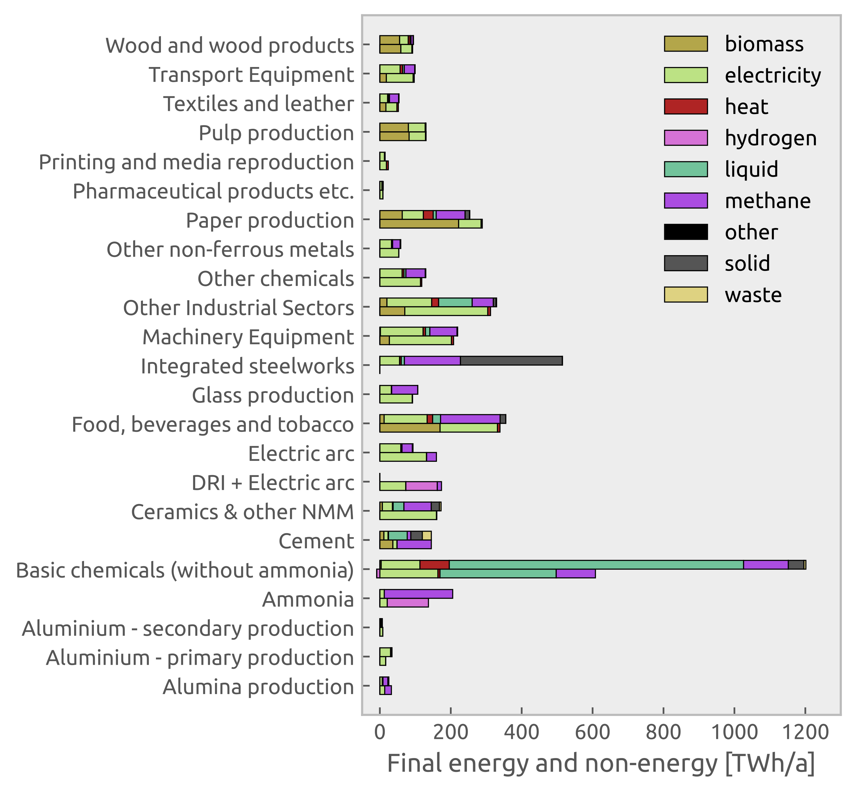
The following figure shows the final consumption of energy and non-energy feedstocks in industry today in comparison to the scenario in 2050 assumed in Neumann et al.
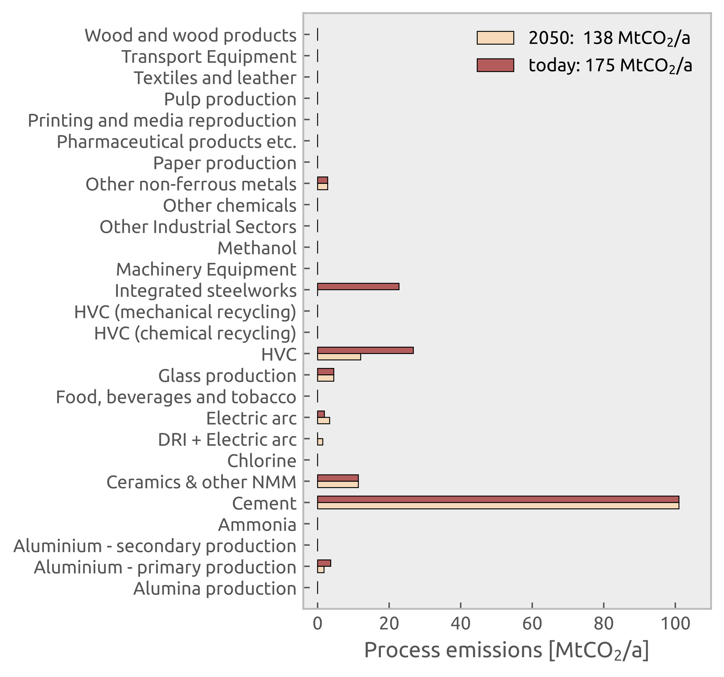
The following figure shows the process emissions in industry today (top bar) and in 2050 without carbon capture (bottom bar) assumed in Neumann et al.
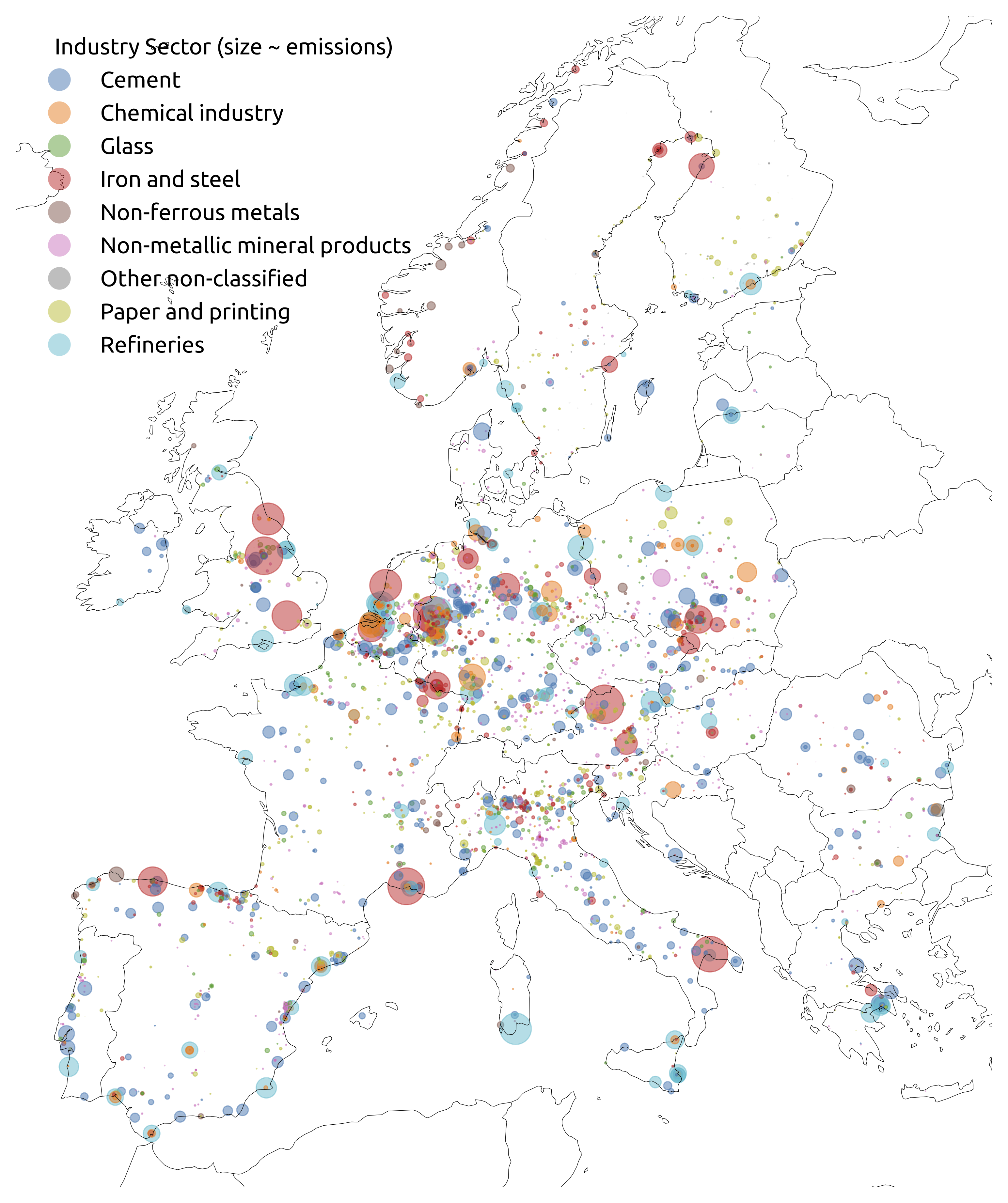
System Message: WARNING/2 (<stdin>, line 5); backlink
Duplicate explicit target name: "hotmaps industrial database".Inside each country the industrial demand is then distributed using the Hotmaps Industrial Database, which is illustrated in the figure below. This open database includes georeferenced industrial sites of energy-intensive industry sectors in EU28, including cement, basic chemicals, glass, iron and steel, non-ferrous metals, non-metallic minerals, paper, and refineries subsectors. The use of this spatial dataset enables the calculation of regional and process-specific energy demands. This approach assumes that there will be no significant migration of energy-intensive industries.
Iron and Steel
Chemicals Industry
The chemicals industry includes a wide range of diverse industries, including the production of basic organic compounds (olefins, alcohols, aromatics), basic inorganic compounds (ammonia, chlorine), polymers (plastics), and end-user products (cosmetics, pharmaceutics).
The chemicals industry includes a wide range of diverse industries, including the production of basic organic compounds (olefins, alcohols, aromatics), basic inorganic compounds (ammonia, chlorine), polymers (plastics), and end-user products (cosmetics, pharmaceutics).
The chemicals industry consumes large amounts of fossil-fuel based feedstocks (see Levi et. al), which can also be produced from renewables as outlined for hydrogen (LINK TO HYDROGEN SUPPLY), for methane (LINK TO METHANE SUPPLY), and for oil-based products (LINK TO OIL-BASED PRODUCTS SUPPLY). The ratio between synthetic and fossil-based fuels used in the industry is an endogenous result of the opti- misation.
The basic chemicals consumption data from the JRC IDEES database comprises high- value chemicals (ethylene, propylene and BTX), chlorine, methanol and ammonia. However, it is necessary to separate out these chemicals because their current and future production routes are different.
Statistics for the production of ammonia, which is commonly used as a fertilizer, are taken from the USGS for every country. Ammonia can be made from hydrogen and nitrogen using the Haber-Bosch process.
$$ N_2 + 3H_2 → 2NH_3 $$
The Haber-Bosch process is not explicitly represented in the model, such that demand for ammonia enters the model as a demand for hydrogen ( $6.5 MWh_{H_2}$ / t $_{NH_3}$ ) and electricity ( $1.17 MWh_{el}$ /t $_{NH_3}$ ) (see Wang et. al). Today, natural gas dominates in Europe as the source for the hydrogen used in the Haber-Bosch process, but the model can choose among the various hydrogen supply options described in the hydrogen section (LINK TO HYDROGEN SUPPLY)
Transportation
Annual energy demands for land transport, aviation and shipping for every country are retrieved from JRC-IDEES data set. Below, the details of how each of these categories are treated is explained.
Land transport
Aviation
The demand for aviation includes international and domestic use. It is modeled as an oil demand since aviation consumes kerosene. This can be produced synthetically or have fossil-origin [link to oil product].
Shipping
System Message: WARNING/2 (<stdin>, line 5); backlink
Duplicate explicit target name: "config file".Shipping energy demand is covered by a combination of oil and hydrogen. The amount of oil products that are converted into hydrogen follow an exogenously defined path. To estimate the hydrogen demand, the average fuel efficiency of the fleet is used in combination with the efficiency of the fuel cell defined in the technology data. The average fuel efficiency is set in the config file.
The consumed hydrogen comes from the general hydrogen bus where it can be produced by SMR, SMR+CC or electrolysers [link to hydrogen]. The fraction that is not converted into hydrogen use oil products, i.e. is connected to the general oil bus.
The user can toggle if the energy demand for liquefaction of the hydrogen used for shipping should be included or not. If this option is selected, liquifaction will happen at the node where the shipping demand occurs.
Carbon dioxide capture, usage and sequestration (CCU/S)
Carbon dioxide can be captured from industry process emissions, emissions related to industry process heat, combined heat and power plants, and directly from the air (DAC).
Carbon dioxide can be used as an input for methanation and Fischer-Tropsch fuels, or it can be sequestered underground.
[Heat demand](#heat-demand)